Key conclusions
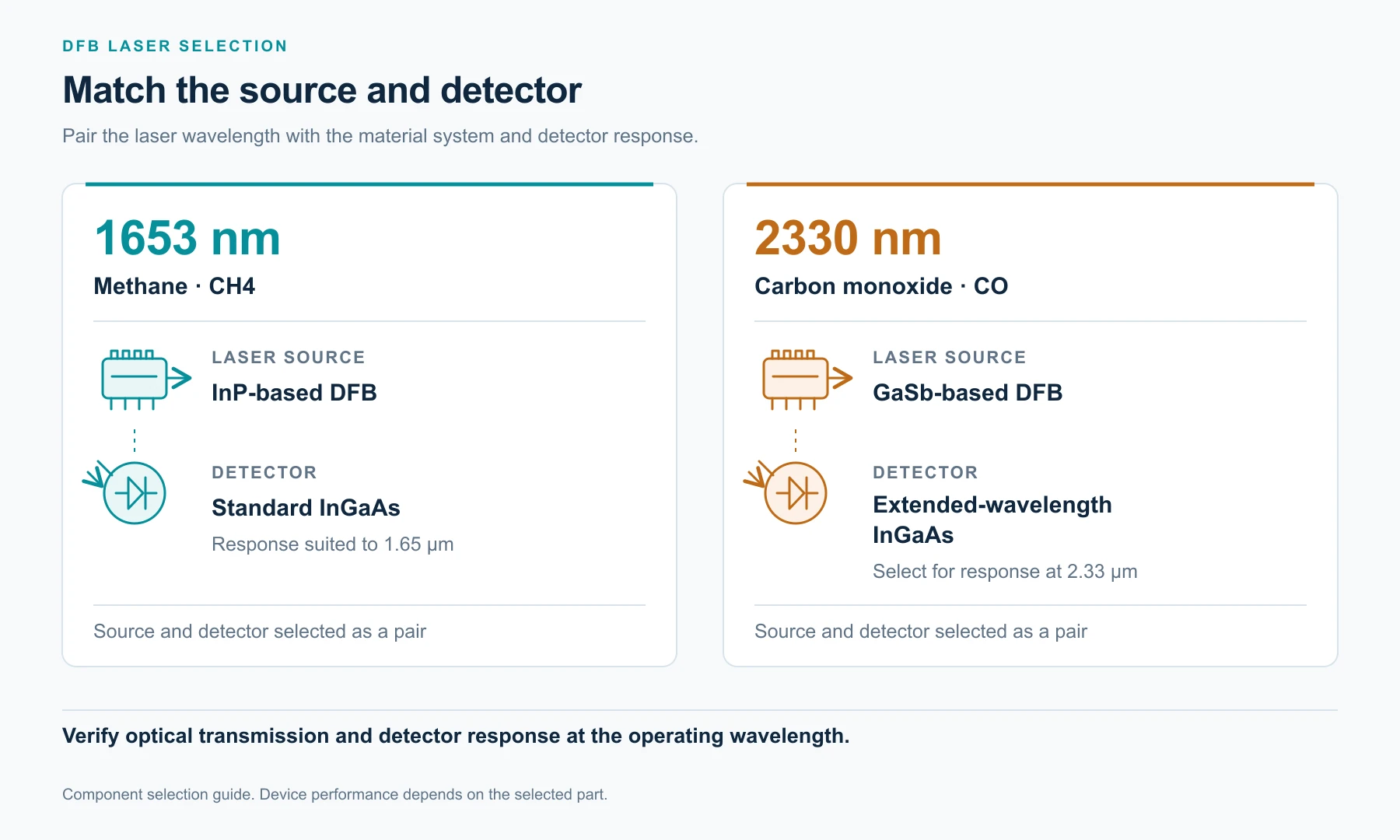
Methane (CH₄) and carbon monoxide (CO) both absorb at several windows between the near- and mid-infrared, but the windows served by single-frequency semiconductor lasers do not coincide. The question this article answers is not which one to pick; it is which band belongs to which gas. The 1653 nm band is the established detection band for methane; the 2330 nm band is the detection band for carbon monoxide. An instrument targeting methane should be built around a 1653 nm source; an instrument targeting CO should be built around a 2330 nm source. Where one instrument must cover both gases, standard practice is two independent sources rather than a single device serving both.
Questions addressed in this article
Where methane's three absorption windows lie | whether 2.3 μm can be used for methane | how much tuning headroom separates the two devices | why 2.33 μm forces a different material system | how sources are configured for simultaneous methane and CO measurement.
1. From three absorption bands to two usable windows
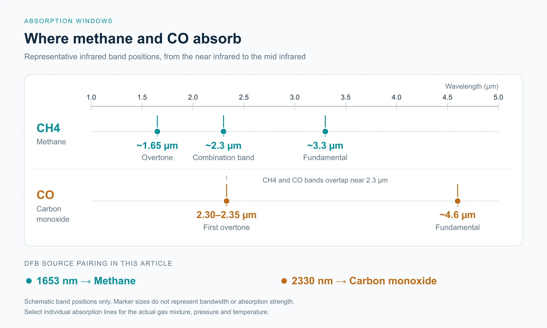
Methane has several absorption bands between 0.8 and 4 μm, of which three are usable in practice. The 3.3 μm band is the C–H stretch fundamental (ν₃) and the strongest. The 1.65 μm band is the 2ν₃ overtone and the weakest. The 2.3 μm region falls on the ν₃+ν₄ combination band, intermediate in strength.
In order of vibrational transition, the fundamental has a substantially larger absorption cross-section than the combination band, which in turn exceeds the overtone by roughly one order of magnitude each step. That ordering is not in dispute spectroscopically.
What that ordering does not settle is the choice of source band. At 3.3 μm there is no usable InP-based diode: InP InGaAs quantum wells stop near 1.7 μm, and extended-wavelength variants near 2.0–2.1 μm. The sources available in this band are antimonide-based type-I diodes, interband cascade lasers (ICL) and quantum cascade lasers (QCL). All three are established at 3.3 μm, and DFB ICLs in particular already run continuous-wave at room temperature in packages close to those of near-infrared DFBs. The difference from the 1653 nm device is not whether it works, but what it costs: cascade structures need higher drive voltage, unit prices exceed those of comparable near-infrared DFBs, lead times are longer and second sources are fewer. For battery-only handheld instruments and mine-warning alarms, where runtime and power are hard constraints, the instrument-level cost and consumption are usually not commercially viable.
The single-frequency distributed feedback (DFB) diodes that are actually available in volume sit at 1.65 μm and 2.3 μm.
The second issue concerns band attribution. The 2.3 μm region does not belong to methane alone. The CO first overtone (2ν) lies at 2.30–2.35 μm and overlaps the methane ν₃+ν₄ combination band in that interval; N₂O lines and weak CO₂ lines are also present. Measuring methane at 2.3 μm is therefore physically possible but requires a prior engineering answer: how far is the selected methane line from the nearest CO line, and what is the ratio of their absorption cross-sections.
At 1.65 μm the situation is reversed. CO has no strong line in this window. The main residual interference comes from weak water-vapour lines, which can be handled by line selection or by drying the sample gas. The methane 2ν₃ overtone, though weak, shows little overlap with coexisting species. Two distinct metrics are involved here. Sensitivity follows from line strength and path length together; selectivity follows from the spacing and strength ratio between the target line and interfering lines. In methane detection, selectivity is usually the binding constraint.
There is a further trade-off on the CO side that deserves a note. CO absorbs most strongly in the 4.6 μm fundamental band, where line strength is roughly two orders of magnitude higher than at the 2.34 μm first overtone. That band requires a QCL or an ICL, carrying the same cost, drive and thermal burden described above for methane at 3.3 μm, and it likewise does not hold up in high-volume, low-cost alarms and portable instruments. The 2ν band at 2.33 μm is therefore a compromise within reach of available diodes, not the strongest choice in principle. This is also why the two devices are selected on different grounds: methane on device maturity, CO on device availability.
2. The two devices compared
| Parameter | GKCP / GKLD-1653-005M-CW-00 | GKLD-2330-003M-CW-00 |
| Centre wavelength | 1653 ± 1 nm | 2325–2333 nm |
| Output power | 5 mW | Not listed in datasheet |
| Wavelength drift | 0.09 nm/°C | 0.2 nm/°C |
| Threshold current | < 20 mA | < 60 mA |
| Operating current | 50 mA | 100 mA |
| Operating voltage | 1.2 V | Not listed in datasheet |
| Emitting width | 2.5 μm | 4 μm |
| Operating temperature | 0–70 °C (25 °C recommended) | 15–35 °C (25 °C recommended) |
| Storage temperature | −40 to 95 °C | −40 to 85 °C |
| Package | Chip (GKCP) or GKLD module | TO-39 ball lens |
| Material system | InP quantum-well ridge-waveguide DFB | GaSb-based DFB |
| Catalogued application | Methane detection, mine gas and domestic alarms | CO detection, domestic alarms, environmental and combustion monitoring |
Table note: data for the 1653 nm device are taken from sections 3.6 (chip, GKCP) and 4.5 (device, GKLD) of the GK Semiconductor product catalogue 0803, and for the 2330 nm device from section 4.7. Entries marked "not listed in datasheet" are gaps in the catalogue, and no estimate is offered here.
What matters most to the system design is wavelength drift, the operating temperature range, and the current headroom above the bias point.
3. Sensitivity and optical path length
Line-strength differences are best stated in orders of magnitude. The 2.3 μm combination band is one to two orders of magnitude above the 1.65 μm overtone, and the 3.3 μm fundamental sits one tier higher again. For any specific transition, the line strength published in HITRAN should be used in the calculation; a ratio quoted in a paper or an article should not be carried over directly.
Under the Beer–Lambert law, absorbance is the product of line strength, concentration and path length. A line one order of magnitude stronger needs one tenth of the path for equal absorbance; two orders stronger needs one hundredth. Three design directions follow.
Instruments with an inherently long path should use 1.65 μm. Open-path perimeter monitoring, fiber-coupled remote heads, in-duct and stack probes, and any structure already built around 10–100 m of optical path. Their constraint is not path length but long-term stability and device cost.
Instruments that need a short path in a fixed installation or with access to mains power may consider 3.3 μm. In-line cells of a few centimeters and process analyzers with mains supply fall into this group. The cost is a more expensive source and a more demanding drive and thermal design. For battery-only handheld devices or drone payloads, power budget and unit price should be checked first; the route is usually not viable, and where it is required at all it presupposes an external supply.
2.3 μm sits between the two. It delivers useful sensitivity over short paths, but the design must also handle CO interference, and it pays off only when line selection is clean.
4. Why 2.33 μm requires a different material system
InP-based strained InGaAs quantum-well lasers available in stable volume reach an emission limit near 2.0–2.1 μm. Extending further into the infrared requires greater strain, at the cost of reliability and lifetime. Reaching 2.33 μm requires a narrower bandgap, which means an antimonide (GaSb-based) or InAs-based system. This follows from band structure, not from sourcing preference.
Three costs follow, and all belong in the system-level budget.
Fewer sources of supply. GaSb DFB epitaxy and chip processing run on dedicated lines rather than as catalogue parts. The main effect is on second-source strategy; the effect on unit price is secondary.
A different detector. Standard InGaAs photodiodes cut off near 1.7 μm. At 2.33 μm an extended-wavelength InGaAs detector is required, with response to 2.6 μm but higher dark current and higher cost. Laser and detector should be budgeted together.
A re-calculated optical train. At 2.3 μm, fused silica sits where the hydroxyl absorption band at 2.22 μm overlaps the infrared absorption tail, so loss is markedly higher than at 1.55 μm and rises quickly with wavelength; bend loss increases as well. Long runs require fluoride fiber or a shortened path, and cannot be extrapolated from 1.55 μm experience. Windows, lenses and filters are available, but the range of catalogue options is markedly smaller than in the near-infrared.
By contrast, the 1.65 μm band inherits the full telecom component ecosystem: single-mode fiber, standard collimators, isolators, WDM filters and process-mature InGaAs detectors, each with a second source. Once a product reaches volume, the value of that ecosystem generally exceeds the advantage in line strength.
5. Tuning headroom: an often omitted specification
TDLAS (tunable diode laser absorption spectroscopy) does not operate statically at a single wavelength. The injection current is modulated so that the wavelength sweeps across the target absorption line, and the sweep range is bounded by the rated operating current.
Two numbers must be kept apart here. The span from threshold to rated current is the device's normal working region, not its scan range. In practice the bias point sits at 70–80 % of rated current, leaving modulation headroom above it; usable scan width is set by the distance from the bias point to the rated limit.
| Part | Threshold current | Rated operating current | Suggested bias point | Current available above bias |
| 1653 nm | < 20 mA | 50 mA | 35–40 mA | 10–15 mA |
| 2330 nm | < 60 mA | 100 mA | 70–80 mA | 20–30 mA |
Table note: the bias point is a drive-design recommendation taken at 70–80 % of the rated current by engineering convention; it is not a device parameter given in the datasheet.
Neither datasheet provides a current-tuning coefficient (dλ/dI), and no industry rule-of-thumb value is used here to derive a scan width. The usable scan width equals the measured tuning coefficient multiplied by the current available above the bias point, and must be characterised on the user's own samples.
Wavelength and frequency are related by Δν ≈ c·Δλ/λ², where c is the speed of light and λ the centre wavelength. At 1653 nm, 1 nm corresponds to about 110 GHz; at 2330 nm, about 55 GHz. A single-frequency DFB tunes over only a fraction of a nanometre within its rated current, so the headroom listed above corresponds to that order of wavelength range: enough to cover one pressure-broadened absorption line, not enough to support multi-line or wide-range measurement. Where an instrument must cover several lines or a broader span, a tunable source such as an external-cavity laser is the appropriate choice, rather than operating a DFB device above its rated current.
6. Thermal control: tighter constraints on the 2330 nm device
Both devices require a thermoelectric cooler (TEC), since both must hold wavelength to a small fraction of the absorption linewidth. The difficulty of doing so differs considerably.
1653 nm device. With a drift coefficient of 0.09 nm/°C across a 0–70 °C operating range. DFB temperature tuning is not linear: mode hops occur across the range, a single hop can reach 0.3–1 nm, and the measured curve is a staircase. The drift over the full range therefore cannot be estimated by multiplying the coefficient by the temperature span, and the usable window should be set from the measured hop boundaries.
At a TEC control accuracy of ±0.1 °C the wavelength is held within about ±0.009 nm, or roughly 1 GHz, about one sixth of the methane linewidth at atmospheric pressure. That is sufficient for ppm-level alarm applications; where relative accuracy of the order of 1 % is required, control should be tightened to the ±0.01 °C level or a reference channel introduced for normalization.
2330 nm device. With a drift coefficient of 0.2 nm/°C across 15–35 °C. That interval is the operating envelope stated in the datasheet, not a recommendation, and the usable window is likewise limited by mode hops. Because the interval spans only 20 °C, ambient temperature must stay inside it at all times; an instrument required to cold-start at −20 °C must heat the laser compartment first.
The narrow window follows from the temperature behaviour of GaSb-based DFBs: threshold current rises and output power falls as temperature increases. It is independent of design quality and belongs in the first structural drawing rather than in the integration phase.
7. Measuring methane and CO in one instrument
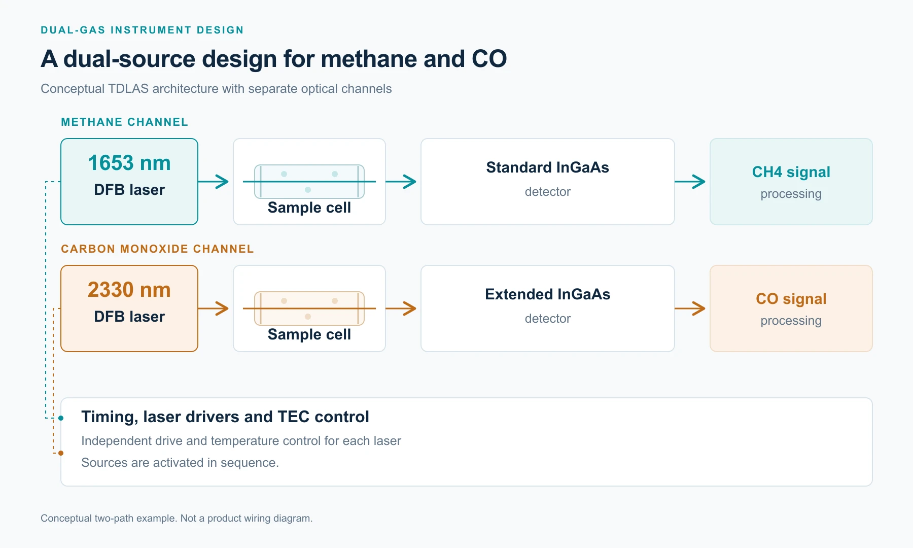
In mining and chemical plant environments the two gases frequently require simultaneous monitoring. Carbon monoxide is colorless and odorless, so its hazard is not readily perceived; piped gas is odorized, which makes a methane leak comparatively easy to notice. Continuous CO monitoring therefore usually carries the stricter requirement.
The standard architecture for such instruments is two sources sharing one optical path or split across two, fired in sequence. The 1653 nm source handles methane with better selectivity; the 2330 nm source handles CO. Both operate near 25 °C off a common thermal and drive schedule. The cost is an additional set of optics, an additional calibration set, and higher overall power consumption.
Attempting to measure both gases with a single 2.33 μm device requires high-resolution spectral retrieval within the overlapping band region, and neither the cost nor the risk is economical.
8. Selection checklist
l Select the target line from HITRAN at the instrument's actual spectral resolution, not from promotional material
l Solve path length and detection limit jointly; avoid fixing the wavelength and back-calculating the path
l For any 2.3 μm design, verify the position and spacing of CO lines either side of the target line
l Match the detector to the band (standard or extended-wavelength InGaAs) with dark current and cost included in the model
l Verify the optical train and any fiber delivery at the actual operating wavelength
l Derive the sweep range from measured dλ/dI, not from a coefficient in the literature
l Confirm that the laser's operating envelope matches the instrument's start-up and storage conditions
l Establish a second-source plan in advance, particularly for antimonide devices
l Explosion-proof and safety certification rests with the instrument manufacturer; source specifications do not constitute system compliance
Frequently asked questions
Which band offers the lower detection limit?
At equal path length, 2.3 μm and 3.3 μm both reach a lower detection limit than 1.65 μm because their line strengths are higher. At equal volume and cost the conclusion does not necessarily hold: a 1.65 μm instrument with a path lengthened to match the line-strength gap can match a 2.3 μm instrument with a short cell. The question is fundamentally one of path design, not wavelength selection.
Can the 2330 nm device be used for methane?
It can, subject to an interference assessment. Methane's combination band and the CO overtone overlap in this region, and poor line selection will read CO as methane. This GK model is catalogued for CO detection and combustion monitoring. Methane use is a custom evaluation requiring line-by-line verification.
Can standard single-mode fiber be used at 2.33 μm?
Over short runs it can be used, but transmission loss rises with wavelength and long-term stability requires separate verification. Measured loss at 2.33 μm should be used as the basis; 1.55 μm data should not be extrapolated.
Why is the operating temperature of the 2330 nm device limited to 15–35 °C?
This follows from the temperature behaviour of GaSb-based DFBs: threshold current rises and output power falls as temperature increases. The datasheet envelope is the range within which the device meets all specifications. If the instrument must operate outside it, the laser compartment requires active heating or insulation.
Is the 2.33 μm device available as a bare die?
The catalogued configuration is a TO-39 ball-lens package. Die-level supply is an engineering question and should be confirmed before designing around a bare chip.